
|
|
|
 View source on GitHub
|
|
This tutorial introduces autoencoders with three examples: the basics, image denoising, and anomaly detection.
An autoencoder is a special type of neural network that is trained to copy its input to its output. For example, given an image of a handwritten digit, an autoencoder first encodes the image into a lower dimensional latent representation, then decodes the latent representation back to an image. An autoencoder learns to compress the data while minimizing the reconstruction error.
To learn more about autoencoders, please consider reading chapter 14 from Deep Learning by Ian Goodfellow, Yoshua Bengio, and Aaron Courville.
Import TensorFlow and other libraries
import matplotlib.pyplot as plt
import numpy as np
import pandas as pd
import tensorflow as tf

from sklearn.metrics import accuracy_score, precision_score, recall_score
from sklearn.model_selection import train_test_split
from tensorflow.keras import layers, losses
from tensorflow.keras.datasets import fashion_mnist
from tensorflow.keras.models import Model
Load the dataset
To start, you will train the basic autoencoder using the Fashion MNIST dataset. Each image in this dataset is 28x28 pixels.
(x_train, _), (x_test, _) = fashion_mnist.load_data()

x_train = x_train.astype('float32') / 255.
x_test = x_test.astype('float32') / 255.

print (x_train.shape)
print (x_test.shape)
Downloading data from https://storage.googleapis.com/tensorflow/tf-keras-datasets/train-labels-idx1-ubyte.gz
29515/29515 ━━━━━━━━━━━━━━━━━━━━ 0s 0us/step
Downloading data from https://storage.googleapis.com/tensorflow/tf-keras-datasets/train-images-idx3-ubyte.gz
26421880/26421880 ━━━━━━━━━━━━━━━━━━━━ 0s 0us/step
Downloading data from https://storage.googleapis.com/tensorflow/tf-keras-datasets/t10k-labels-idx1-ubyte.gz
5148/5148 ━━━━━━━━━━━━━━━━━━━━ 0s 0us/step
Downloading data from https://storage.googleapis.com/tensorflow/tf-keras-datasets/t10k-images-idx3-ubyte.gz
4422102/4422102 ━━━━━━━━━━━━━━━━━━━━ 0s 0us/step
(60000, 28, 28)
(10000, 28, 28)
First example: Basic autoencoder
Define an autoencoder with two Dense layers: an encoder, which compresses the images into a 64 dimensional latent vector, and a decoder, that reconstructs the original image from the latent space.
To define your model, use the Keras Model Subclassing API.
class Autoencoder(Model):
  def __init__(self, latent_dim, shape):
    super(Autoencoder, self).__init__()
    self.latent_dim = latent_dim
    self.shape = shape
    self.encoder = tf.keras.Sequential([
      layers.Flatten(),
      layers.Dense(latent_dim, activation='relu'),
    ])
    self.decoder = tf.keras.Sequential([
      layers.Dense(tf.math.reduce_prod(shape).numpy(), activation='sigmoid'),
      layers.Reshape(shape)
    ])

  def call(self, x):
    encoded = self.encoder(x)
    decoded = self.decoder(encoded)
    return decoded


shape = x_test.shape[1:]
latent_dim = 64
autoencoder = Autoencoder(latent_dim, shape)
autoencoder.compile(optimizer='adam', loss=losses.MeanSquaredError())
Train the model using x_train as both the input and the target. The encoder will learn to compress the dataset from 784 dimensions to the latent space, and the decoder will learn to reconstruct the original images.
.
autoencoder.fit(x_train, x_train,
                epochs=10,
                shuffle=True,
                validation_data=(x_test, x_test))
Epoch 1/10
WARNING: All log messages before absl::InitializeLog() is called are written to STDERR
I0000 00:00:1713230807.172583   14227 service.cc:145] XLA service 0x7fe4cc007e20 initialized for platform CUDA (this does not guarantee that XLA will be used). Devices:
I0000 00:00:1713230807.172638   14227 service.cc:153]   StreamExecutor device (0): Tesla T4, Compute Capability 7.5
I0000 00:00:1713230807.172643   14227 service.cc:153]   StreamExecutor device (1): Tesla T4, Compute Capability 7.5
I0000 00:00:1713230807.172646   14227 service.cc:153]   StreamExecutor device (2): Tesla T4, Compute Capability 7.5
I0000 00:00:1713230807.172648   14227 service.cc:153]   StreamExecutor device (3): Tesla T4, Compute Capability 7.5
131/1875 ━━━━━━━━━━━━━━━━━━━━ 2s 1ms/step - loss: 0.1034
I0000 00:00:1713230807.858362   14227 device_compiler.h:188] Compiled cluster using XLA!  This line is logged at most once for the lifetime of the process.
1875/1875 ━━━━━━━━━━━━━━━━━━━━ 5s 2ms/step - loss: 0.0397 - val_loss: 0.0134
Epoch 2/10
1875/1875 ━━━━━━━━━━━━━━━━━━━━ 2s 1ms/step - loss: 0.0124 - val_loss: 0.0111
Epoch 3/10
1875/1875 ━━━━━━━━━━━━━━━━━━━━ 3s 1ms/step - loss: 0.0102 - val_loss: 0.0097
Epoch 4/10
1875/1875 ━━━━━━━━━━━━━━━━━━━━ 2s 1ms/step - loss: 0.0095 - val_loss: 0.0094
Epoch 5/10
1875/1875 ━━━━━━━━━━━━━━━━━━━━ 2s 1ms/step - loss: 0.0092 - val_loss: 0.0092
Epoch 6/10
1875/1875 ━━━━━━━━━━━━━━━━━━━━ 3s 1ms/step - loss: 0.0090 - val_loss: 0.0090
Epoch 7/10
1875/1875 ━━━━━━━━━━━━━━━━━━━━ 2s 1ms/step - loss: 0.0089 - val_loss: 0.0089
Epoch 8/10
1875/1875 ━━━━━━━━━━━━━━━━━━━━ 2s 1ms/step - loss: 0.0088 - val_loss: 0.0090
Epoch 9/10
1875/1875 ━━━━━━━━━━━━━━━━━━━━ 2s 1ms/step - loss: 0.0087 - val_loss: 0.0089
Epoch 10/10
1875/1875 ━━━━━━━━━━━━━━━━━━━━ 2s 1ms/step - loss: 0.0087 - val_loss: 0.0088
<keras.src.callbacks.history.History at 0x7fe6854d9b50>
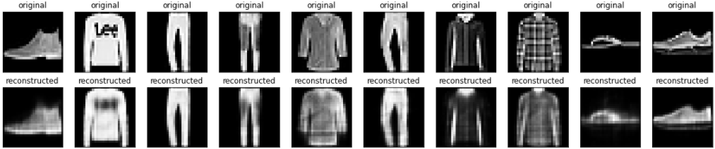
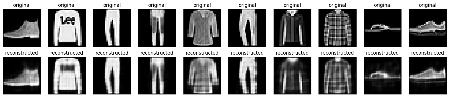
Now that the model is trained, let's test it by encoding and decoding images from the test set.
encoded_imgs = autoencoder.encoder(x_test).numpy()
decoded_imgs = autoencoder.decoder(encoded_imgs).numpy()
n = 10
plt.figure(figsize=(20, 4))
for i in range(n):
  # display original
  ax = plt.subplot(2, n, i + 1)
  plt.imshow(x_test[i])
  plt.title("original")
  plt.gray()
  ax.get_xaxis().set_visible(False)
  ax.get_yaxis().set_visible(False)

  # display reconstruction
  ax = plt.subplot(2, n, i + 1 + n)
  plt.imshow(decoded_imgs[i])
  plt.title("reconstructed")
  plt.gray()
  ax.get_xaxis().set_visible(False)
  ax.get_yaxis().set_visible(False)
plt.show()
Second example: Image denoising
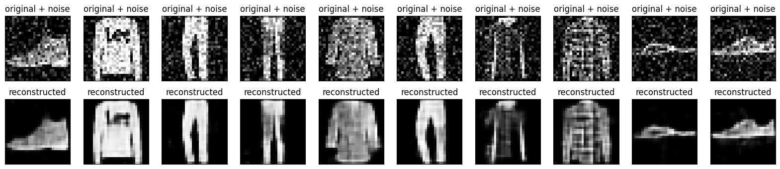
An autoencoder can also be trained to remove noise from images. In the following section, you will create a noisy version of the Fashion MNIST dataset by applying random noise to each image. You will then train an autoencoder using the noisy image as input, and the original image as the target.
Let's reimport the dataset to omit the modifications made earlier.
(x_train, _), (x_test, _) = fashion_mnist.load_data()
x_train = x_train.astype('float32') / 255.
x_test = x_test.astype('float32') / 255.

x_train = x_train[..., tf.newaxis]
x_test = x_test[..., tf.newaxis]

print(x_train.shape)
(60000, 28, 28, 1)
Adding random noise to the images
noise_factor = 0.2
x_train_noisy = x_train + noise_factor * tf.random.normal(shape=x_train.shape)
x_test_noisy = x_test + noise_factor * tf.random.normal(shape=x_test.shape)

x_train_noisy = tf.clip_by_value(x_train_noisy, clip_value_min=0., clip_value_max=1.)
x_test_noisy = tf.clip_by_value(x_test_noisy, clip_value_min=0., clip_value_max=1.)
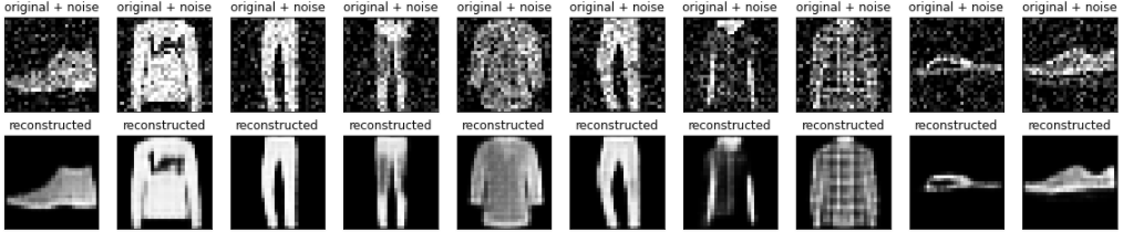
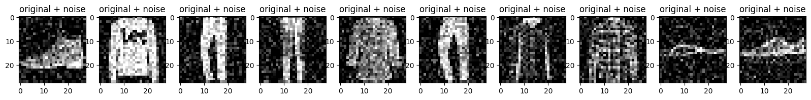
Plot the noisy images.
n = 10
plt.figure(figsize=(20, 2))
for i in range(n):
    ax = plt.subplot(1, n, i + 1)
    plt.title("original + noise")
    plt.imshow(tf.squeeze(x_test_noisy[i]))
    plt.gray()
plt.show()
Define a convolutional autoencoder
In this example, you will train a convolutional autoencoder using Conv2D layers in the encoder, and Conv2DTranspose layers in the decoder.
class Denoise(Model):
  def __init__(self):
    super(Denoise, self).__init__()
    self.encoder = tf.keras.Sequential([
      layers.Input(shape=(28, 28, 1)),
      layers.Conv2D(16, (3, 3), activation='relu', padding='same', strides=2),
      layers.Conv2D(8, (3, 3), activation='relu', padding='same', strides=2)])

    self.decoder = tf.keras.Sequential([
      layers.Conv2DTranspose(8, kernel_size=3, strides=2, activation='relu', padding='same'),
      layers.Conv2DTranspose(16, kernel_size=3, strides=2, activation='relu', padding='same'),
      layers.Conv2D(1, kernel_size=(3, 3), activation='sigmoid', padding='same')])

  def call(self, x):
    encoded = self.encoder(x)
    decoded = self.decoder(encoded)
    return decoded

autoencoder = Denoise()
autoencoder.compile(optimizer='adam', loss=losses.MeanSquaredError())
autoencoder.fit(x_train_noisy, x_train,
                epochs=10,
                shuffle=True,
                validation_data=(x_test_noisy, x_test))
Epoch 1/10
1875/1875 ━━━━━━━━━━━━━━━━━━━━ 7s 2ms/step - loss: 0.0332 - val_loss: 0.0094
Epoch 2/10
1875/1875 ━━━━━━━━━━━━━━━━━━━━ 3s 2ms/step - loss: 0.0089 - val_loss: 0.0081
Epoch 3/10
1875/1875 ━━━━━━━━━━━━━━━━━━━━ 4s 2ms/step - loss: 0.0079 - val_loss: 0.0076
Epoch 4/10
1875/1875 ━━━━━━━━━━━━━━━━━━━━ 4s 2ms/step - loss: 0.0074 - val_loss: 0.0073
Epoch 5/10
1875/1875 ━━━━━━━━━━━━━━━━━━━━ 4s 2ms/step - loss: 0.0072 - val_loss: 0.0071
Epoch 6/10
1875/1875 ━━━━━━━━━━━━━━━━━━━━ 4s 2ms/step - loss: 0.0070 - val_loss: 0.0070
Epoch 7/10
1875/1875 ━━━━━━━━━━━━━━━━━━━━ 4s 2ms/step - loss: 0.0069 - val_loss: 0.0069
Epoch 8/10
1875/1875 ━━━━━━━━━━━━━━━━━━━━ 4s 2ms/step - loss: 0.0068 - val_loss: 0.0068
Epoch 9/10
1875/1875 ━━━━━━━━━━━━━━━━━━━━ 4s 2ms/step - loss: 0.0068 - val_loss: 0.0067
Epoch 10/10
1875/1875 ━━━━━━━━━━━━━━━━━━━━ 3s 2ms/step - loss: 0.0067 - val_loss: 0.0067
<keras.src.callbacks.history.History at 0x7fe6883e5a30>
Let's take a look at a summary of the encoder. Notice how the images are downsampled from 28x28 to 7x7.
autoencoder.encoder.summary()
The decoder upsamples the images back from 7x7 to 28x28.
autoencoder.decoder.summary()
Plotting both the noisy images and the denoised images produced by the autoencoder.
encoded_imgs = autoencoder.encoder(x_test_noisy).numpy()
decoded_imgs = autoencoder.decoder(encoded_imgs).numpy()
n = 10
plt.figure(figsize=(20, 4))
for i in range(n):

    # display original + noise
    ax = plt.subplot(2, n, i + 1)
    plt.title("original + noise")
    plt.imshow(tf.squeeze(x_test_noisy[i]))
    plt.gray()
    ax.get_xaxis().set_visible(False)
    ax.get_yaxis().set_visible(False)

    # display reconstruction
    bx = plt.subplot(2, n, i + n + 1)
    plt.title("reconstructed")
    plt.imshow(tf.squeeze(decoded_imgs[i]))
    plt.gray()
    bx.get_xaxis().set_visible(False)
    bx.get_yaxis().set_visible(False)
plt.show()
Third example: Anomaly detection
Overview
In this example, you will train an autoencoder to detect anomalies on the ECG5000 dataset. This dataset contains 5,000 Electrocardiograms, each with 140 data points. You will use a simplified version of the dataset, where each example has been labeled either 0 (corresponding to an abnormal rhythm), or 1 (corresponding to a normal rhythm). You are interested in identifying the abnormal rhythms.
How will you detect anomalies using an autoencoder? Recall that an autoencoder is trained to minimize reconstruction error. You will train an autoencoder on the normal rhythms only, then use it to reconstruct all the data. Our hypothesis is that the abnormal rhythms will have higher reconstruction error. You will then classify a rhythm as an anomaly if the reconstruction error surpasses a fixed threshold.
Load ECG data
The dataset you will use is based on one from timeseriesclassification.com.
# Download the dataset
dataframe = pd.read_csv('http://storage.googleapis.com/download.tensorflow.org/data/ecg.csv', header=None)
raw_data = dataframe.values
dataframe.head()
# The last element contains the labels
labels = raw_data[:, -1]

# The other data points are the electrocadriogram data
data = raw_data[:, 0:-1]

train_data, test_data, train_labels, test_labels = train_test_split(
    data, labels, test_size=0.2, random_state=21
)
Normalize the data to [0,1].
min_val = tf.reduce_min(train_data)
max_val = tf.reduce_max(train_data)

train_data = (train_data - min_val) / (max_val - min_val)
test_data = (test_data - min_val) / (max_val - min_val)

train_data = tf.cast(train_data, tf.float32)
test_data = tf.cast(test_data, tf.float32)
You will train the autoencoder using only the normal rhythms, which are labeled in this dataset as 1. Separate the normal rhythms from the abnormal rhythms.
train_labels = train_labels.astype(bool)
test_labels = test_labels.astype(bool)

normal_train_data = train_data[train_labels]
normal_test_data = test_data[test_labels]

anomalous_train_data = train_data[~train_labels]
anomalous_test_data = test_data[~test_labels]
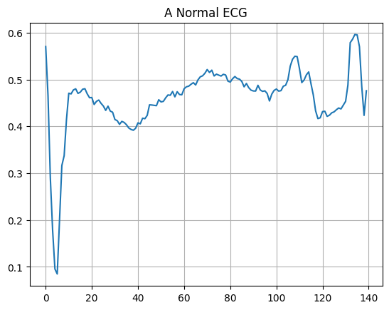
Plot a normal ECG.
plt.grid()
plt.plot(np.arange(140), normal_train_data[0])
plt.title("A Normal ECG")
plt.show()
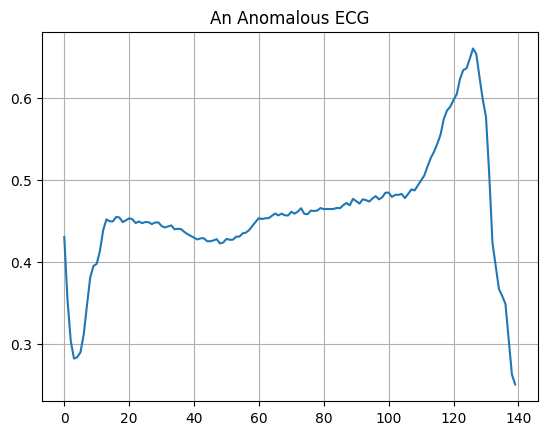
Plot an anomalous ECG.
plt.grid()
plt.plot(np.arange(140), anomalous_train_data[0])
plt.title("An Anomalous ECG")
plt.show()
Build the model
class AnomalyDetector(Model):
  def __init__(self):
    super(AnomalyDetector, self).__init__()
    self.encoder = tf.keras.Sequential([
      layers.Dense(32, activation="relu"),
      layers.Dense(16, activation="relu"),
      layers.Dense(8, activation="relu")])

    self.decoder = tf.keras.Sequential([
      layers.Dense(16, activation="relu"),
      layers.Dense(32, activation="relu"),
      layers.Dense(140, activation="sigmoid")])

  def call(self, x):
    encoded = self.encoder(x)
    decoded = self.decoder(encoded)
    return decoded

autoencoder = AnomalyDetector()
autoencoder.compile(optimizer='adam', loss='mae')
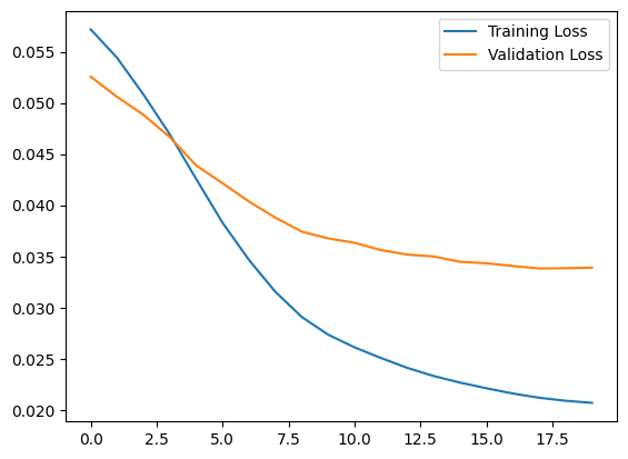
Notice that the autoencoder is trained using only the normal ECGs, but is evaluated using the full test set.
history = autoencoder.fit(normal_train_data, normal_train_data,
          epochs=20,
          batch_size=512,
          validation_data=(test_data, test_data),
          shuffle=True)
Epoch 1/20
5/5 ━━━━━━━━━━━━━━━━━━━━ 5s 494ms/step - loss: 0.0575 - val_loss: 0.0526
Epoch 2/20
5/5 ━━━━━━━━━━━━━━━━━━━━ 0s 14ms/step - loss: 0.0549 - val_loss: 0.0506
Epoch 3/20
5/5 ━━━━━━━━━━━━━━━━━━━━ 0s 13ms/step - loss: 0.0514 - val_loss: 0.0488
Epoch 4/20
5/5 ━━━━━━━━━━━━━━━━━━━━ 0s 13ms/step - loss: 0.0475 - val_loss: 0.0466
Epoch 5/20
5/5 ━━━━━━━━━━━━━━━━━━━━ 0s 14ms/step - loss: 0.0432 - val_loss: 0.0439
Epoch 6/20
5/5 ━━━━━━━━━━━━━━━━━━━━ 0s 13ms/step - loss: 0.0389 - val_loss: 0.0421
Epoch 7/20
5/5 ━━━━━━━━━━━━━━━━━━━━ 0s 13ms/step - loss: 0.0353 - val_loss: 0.0404
Epoch 8/20
5/5 ━━━━━━━━━━━━━━━━━━━━ 0s 13ms/step - loss: 0.0319 - val_loss: 0.0388
Epoch 9/20
5/5 ━━━━━━━━━━━━━━━━━━━━ 0s 14ms/step - loss: 0.0290 - val_loss: 0.0374
Epoch 10/20
5/5 ━━━━━━━━━━━━━━━━━━━━ 0s 13ms/step - loss: 0.0276 - val_loss: 0.0368
Epoch 11/20
5/5 ━━━━━━━━━━━━━━━━━━━━ 0s 14ms/step - loss: 0.0264 - val_loss: 0.0363
Epoch 12/20
5/5 ━━━━━━━━━━━━━━━━━━━━ 0s 14ms/step - loss: 0.0254 - val_loss: 0.0356
Epoch 13/20
5/5 ━━━━━━━━━━━━━━━━━━━━ 0s 13ms/step - loss: 0.0242 - val_loss: 0.0352
Epoch 14/20
5/5 ━━━━━━━━━━━━━━━━━━━━ 0s 14ms/step - loss: 0.0234 - val_loss: 0.0350
Epoch 15/20
5/5 ━━━━━━━━━━━━━━━━━━━━ 0s 14ms/step - loss: 0.0229 - val_loss: 0.0345
Epoch 16/20
5/5 ━━━━━━━━━━━━━━━━━━━━ 0s 14ms/step - loss: 0.0222 - val_loss: 0.0343
Epoch 17/20
5/5 ━━━━━━━━━━━━━━━━━━━━ 0s 13ms/step - loss: 0.0216 - val_loss: 0.0341
Epoch 18/20
5/5 ━━━━━━━━━━━━━━━━━━━━ 0s 14ms/step - loss: 0.0212 - val_loss: 0.0338
Epoch 19/20
5/5 ━━━━━━━━━━━━━━━━━━━━ 0s 14ms/step - loss: 0.0210 - val_loss: 0.0338
Epoch 20/20
5/5 ━━━━━━━━━━━━━━━━━━━━ 0s 14ms/step - loss: 0.0208 - val_loss: 0.0339
plt.plot(history.history["loss"], label="Training Loss")
plt.plot(history.history["val_loss"], label="Validation Loss")
plt.legend()
<matplotlib.legend.Legend at 0x7fe6704c3520>
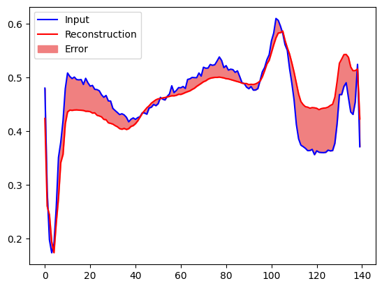
You will soon classify an ECG as anomalous if the reconstruction error is greater than one standard deviation from the normal training examples. First, let's plot a normal ECG from the training set, the reconstruction after it's encoded and decoded by the autoencoder, and the reconstruction error.
encoded_data = autoencoder.encoder(normal_test_data).numpy()
decoded_data = autoencoder.decoder(encoded_data).numpy()

plt.plot(normal_test_data[0], 'b')
plt.plot(decoded_data[0], 'r')
plt.fill_between(np.arange(140), decoded_data[0], normal_test_data[0], color='lightcoral')
plt.legend(labels=["Input", "Reconstruction", "Error"])
plt.show()
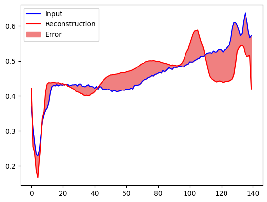
Create a similar plot, this time for an anomalous test example.
encoded_data = autoencoder.encoder(anomalous_test_data).numpy()
decoded_data = autoencoder.decoder(encoded_data).numpy()

plt.plot(anomalous_test_data[0], 'b')
plt.plot(decoded_data[0], 'r')
plt.fill_between(np.arange(140), decoded_data[0], anomalous_test_data[0], color='lightcoral')
plt.legend(labels=["Input", "Reconstruction", "Error"])
plt.show()
Detect anomalies
Detect anomalies by calculating whether the reconstruction loss is greater than a fixed threshold. In this tutorial, you will calculate the mean average error for normal examples from the training set, then classify future examples as anomalous if the reconstruction error is higher than one standard deviation from the training set.
Plot the reconstruction error on normal ECGs from the training set
reconstructions = autoencoder.predict(normal_train_data)
train_loss = tf.keras.losses.mae(reconstructions, normal_train_data)

plt.hist(train_loss[None,:], bins=50)
plt.xlabel("Train loss")
plt.ylabel("No of examples")
plt.show()
74/74 ━━━━━━━━━━━━━━━━━━━━ 1s 6ms/step
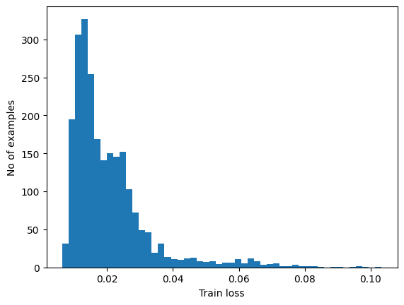
Choose a threshold value that is one standard deviations above the mean.
threshold = np.mean(train_loss) + np.std(train_loss)
print("Threshold: ", threshold)
Threshold: 0.033047937
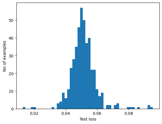
If you examine the reconstruction error for the anomalous examples in the test set, you'll notice most have greater reconstruction error than the threshold. By varing the threshold, you can adjust the precision and recall of your classifier.
reconstructions = autoencoder.predict(anomalous_test_data)
test_loss = tf.keras.losses.mae(reconstructions, anomalous_test_data)

plt.hist(test_loss[None, :], bins=50)
plt.xlabel("Test loss")
plt.ylabel("No of examples")
plt.show()
14/14 ━━━━━━━━━━━━━━━━━━━━ 0s 22ms/step
Classify an ECG as an anomaly if the reconstruction error is greater than the threshold.
def predict(model, data, threshold):
  reconstructions = model(data)
  loss = tf.keras.losses.mae(reconstructions, data)
  return tf.math.less(loss, threshold)

def print_stats(predictions, labels):
  print("Accuracy = {}".format(accuracy_score(labels, predictions)))
  print("Precision = {}".format(precision_score(labels, predictions)))
  print("Recall = {}".format(recall_score(labels, predictions)))
preds = predict(autoencoder, test_data, threshold)
print_stats(preds, test_labels)
Accuracy = 0.944
Precision = 0.9921875
Recall = 0.9071428571428571
Next steps
To learn more about anomaly detection with autoencoders, check out this excellent interactive example built with TensorFlow.js by Victor Dibia. For a real-world use case, you can learn how Airbus Detects Anomalies in ISS Telemetry Data using TensorFlow. To learn more about the basics, consider reading this blog post by François Chollet. For more details, check out chapter 14 from Deep Learning by Ian Goodfellow, Yoshua Bengio, and Aaron Courville.